Decoding Rotary Positional Embeddings (RoPE)

I've been digging into the source code of a few modern LLMs lately, and RoPE or Rotary Positional Embedding is everywhere. I knew it was a replacement for the original sinusoidal or learned absolute position embeddings, but I didn't have a clear idea on the how or the why. So, I decided to go down the rabbit hole. These are my notes.

First Contact: What's the Big Idea?

My initial understanding was that instead of adding a positional vector to the token embedding, RoPE modifies the query and key vectors in the attention mechanism. The original paper's claim is that it encodes positional information in a relative way.

Start with a 2-D Vector

Let's say we have a 2-D vector \(x = [x_1, x_2]\). This vector represents a single dimension pair from a larger embedding vector.

Define the Rotation

The rotation for RoPE is defined by a matrix. For a pair of dimensions at a specific position \(m\), the rotation matrix \(R_m\) is:

$$ R_m = \begin{bmatrix} \cos(m\theta) & -\sin(m\theta) \\ \sin(m\theta) & \cos(m\theta) \end{bmatrix} $$

Here, \(\theta\) is a constant that is different for each pair of dimensions. Typically, \(\theta_j = 10000^{-2j/d}\) where \(j\) is the dimension index and \(d\) is the total dimension of the embedding.

Apply the Rotation

The transformed vector \(x'_m\) at position \(m\) is calculated by multiplying the original vector \(x\) by the rotation matrix \(R_m\):

$$ x'_m = R_m x = \begin{bmatrix} \cos(m\theta) & -\sin(m\theta) \\ \sin(m\theta) & \cos(m\theta) \end{bmatrix} \begin{bmatrix} x_1 \\ x_2 \end{bmatrix} $$

This gives us the new, rotated vector:

$$ x'_m = \begin{bmatrix} x_1 \cos(m\theta) - x_2 \sin(m\theta) \\ x_1 \sin(m\theta) + x_2 \cos(m\theta) \end{bmatrix} $$

This is the core of how RoPE works: it rotates the vector by an angle \(m\theta\).

Making Sense of the Math and Frequencies

The angle for each rotation depends on the token's position m and the dimension pair's index j. The formula for the base rotational "speed" is:

θj = 10000(-2j/d)

Here, d is the head dimension. For a model like the Gemma3 270M, d is 256. This means j, the index of the feature pair, runs from 0 to 127 (since d/2 - 1 = 127). To better understand what this looked like, I plotted it. Words and formulas only get you so far.

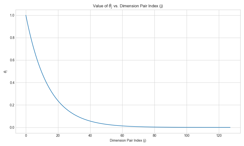
This is the plot of θj against the dimension pair index j for d=256:

The plot showed a clear exponential decay. The first few dimension pairs have high frequencies (large θ), meaning they rotate fast. The later pairs have low frequencies, rotating very slowly. This multi-frequency approach seems key to encoding position at different resolutions.

How Relative Distance Changes

To wrap my head around the "relative" part, I plotted the cosine scaling factor that RoPE applies to the dot product for different relative distances. This factor depends on the relative distance m-n.

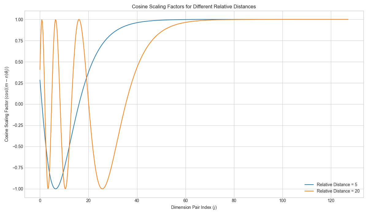
Here are five key opinions and interpretations drawn from it:

1. Unique Rotational Signatures for Each Distance. The most apparent takeaway is that different relative distances produce entirely different curves. The orange curve (distance = 20) oscillates far more rapidly in the initial dimensions than the blue curve (distance = 5). This illustrates the fundamental principle of RoPE: it encodes the relative distance between tokens into a unique rotational "signature," allowing the model to distinguish between tokens that are 5 positions apart versus 20 positions apart.
2. High-Frequency Dimensions Encode Fine-Grained Position. The plot reveals that all the complex, wave-like behavior is concentrated in the early "Dimension Pair Index" values (the high-frequency dimensions). These dimensions are highly sensitive to changes in position and are therefore specialized for encoding the precise relative location of tokens. As the distance increases, the rotations in these dimensions become faster and more pronounced.
3. Long-Distance Attention Decay. For the larger relative distance (orange line), the cosine factor fluctuates dramatically between -1 and 1. When the model aggregates these values across dimensions to compute an attention score, these rapid oscillations tend to cancel each other out. This naturally causes the attention score to "decay" over longer distances, a desirable property that encourages the model to prioritize more local context.
4. Low-Frequency Dimensions Preserve Content. In contrast, for higher dimension pair indices (roughly 60 and above), both curves converge and flatten out at 1.0. This is crucial because it means these low-frequency dimensions are effectively "ignoring" the positional information. By keeping the scaling factor at 1, RoPE ensures that the original, content-based meaning of the token embeddings is preserved in this part of the vector space, allowing the model to attend to words based on what they mean, not just where they are.
5. Analogy: A "Filter Bank" for Warranted Attention. The behavior of the curves lends itself well to a "filter bank" analogy. Each dimension pair acts as a filter that tests the relationship between two tokens. For a large relative distance, the rapid oscillations create a very stringent set of filters. For attention to be high, the semantic connection between the words must be strong enough to overcome the many negative positional scores from these filters. In this view, long-distance attention is only granted when it is truly "warranted," ensuring that the model forms meaningful long-range connections instead of spurious ones.

The Implementation Rabbit Hole: Two Styles Emerged

This is where things got really interesting. Once I felt I had a handle on the theory, I looked at how it was implemented in code. The first version I found was super clean:

Style 1: The Half-and-Half Split

I first came across this style in the Gemma source code. It's a very direct approach: the vector is split cleanly into two halves, x1 and x2, which are then combined to perform the rotation. I noticed that Qwen and GPT-OSS use a similar, straightforward implementation.

# Qwen / Gemma /GPT-OSS style
def rotate_half(x):
    x1 = x[..., : x.shape[-1] // 2]
    x2 = x[..., x.shape[-1] // 2 :]
    return torch.cat((-x2, x1), dim=-1)

def apply_rotary_pos_emb(q, k, cos, sin):
    ...
    q_embed = (q * cos) + (rotate_half(q) * sin)
    k_embed = (k * cos) + (rotate_half(k) * sin)
    return q_embed, k_embed
                    

This implementation was intuitive. It pairs the i-th element of the first half with the i-th element of the second half.

Style 2: The Interleaved Pairing

However, the original RoPE paper described an interleaved pairing method. When I checked the Llama implementation on Hugging Face, I saw it used this exact approach, as did GLM-4. Instead of a simple half-and-half split, this method uses slicing with a step of 2 to select alternating elements.

# GLM-4 / Llama style
def rotate_half(x):
    # This pairs (x0, x1), (x2, x3), etc.
    x1 = x[..., 0::2]
    x2 = x[..., 1::2]
    return torch.stack((-x2, x1), dim=-1).flatten(-2)

def apply_rotary_pos_emb(q, k, cos, sin):
    # This cos/sin needs to be prepared differently too, often with repeat_interleave
    # ...
    q_embed = (q * cos) + (rotate_half(q) * sin)
    k_embed = (k * cos) + (rotate_half(k) * sin)
    return q_embed, k_embed
                    

This was a little confusing at first. It took me a moment to grasp that it's just a different way of pairing up the dimensions for rotation. Instead of pairing (x_i, x_{i + d/2}) like the first style, this one pairs adjacent elements: (x₀, x₁), (x₂, x₃), and so on. Ultimately, both methods achieve the same goal of creating the d/2 2D subspaces needed for rotation—they just group the dimensions differently.

This whole exercise was super valuable. It started with a confusing acronym in a config file and ended with a much deeper appreciation for the elegance of the solution. It also served as a good reminder that there are often multiple ways to implement the same core mathematical idea, and checking the source code of different models is crucial for a complete picture.